Note
Go to the end to download the full example code or to run this example in your browser via JupyterLite or Binder.
Balance model complexity and cross-validated score#
This example demonstrates how to balance model complexity and cross-validated score by
finding a decent accuracy within 1 standard deviation of the best accuracy score while
minimising the number of PCA components [1]. It uses
GridSearchCV with a custom refit callable to select
the optimal model.
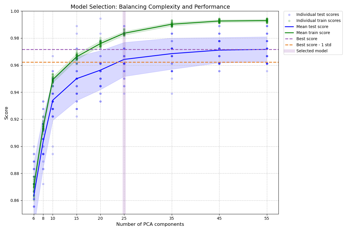
The figure shows the trade-off between cross-validated score and the number
of PCA components. The balanced case is when n_components=10 and accuracy=0.88,
which falls into the range within 1 standard deviation of the best accuracy
score.
References#
# Authors: The scikit-learn developers
# SPDX-License-Identifier: BSD-3-Clause

import matplotlib.pyplot as plt
import numpy as np
import polars as pl

from sklearn.datasets import load_digits
from sklearn.decomposition import PCA
from sklearn.linear_model import LogisticRegression
from sklearn.model_selection import GridSearchCV, ShuffleSplit
from sklearn.pipeline import Pipeline
Introduction#
When tuning hyperparameters, we often want to balance model complexity and performance. The “one-standard-error” rule is a common approach: select the simplest model whose performance is within one standard error of the best model’s performance. This helps to avoid overfitting by preferring simpler models when their performance is statistically comparable to more complex ones.
Helper functions#
We define two helper functions:
lower_bound: Calculates the threshold for acceptable performance (best score - 1 std)best_low_complexity: Selects the model with the fewest PCA components that exceeds this threshold
def lower_bound(cv_results):
    """
    Calculate the lower bound within 1 standard deviation
    of the best `mean_test_scores`.

    Parameters
    ----------
    cv_results : dict of numpy(masked) ndarrays
        See attribute cv_results_ of `GridSearchCV`

    Returns
    -------
    float
        Lower bound within 1 standard deviation of the
        best `mean_test_score`.
    """
    best_score_idx = np.argmax(cv_results["mean_test_score"])

    return (
        cv_results["mean_test_score"][best_score_idx]
        - cv_results["std_test_score"][best_score_idx]
    )


def best_low_complexity(cv_results):
    """
    Balance model complexity with cross-validated score.

    Parameters
    ----------
    cv_results : dict of numpy(masked) ndarrays
        See attribute cv_results_ of `GridSearchCV`.

    Return
    ------
    int
        Index of a model that has the fewest PCA components
        while has its test score within 1 standard deviation of the best
        `mean_test_score`.
    """
    threshold = lower_bound(cv_results)
    candidate_idx = np.flatnonzero(cv_results["mean_test_score"] >= threshold)
    best_idx = candidate_idx[
        cv_results["param_reduce_dim__n_components"][candidate_idx].argmin()
    ]
    return best_idx
Set up the pipeline and parameter grid#
We create a pipeline with two steps:
Dimensionality reduction using PCA
Classification using LogisticRegression
We’ll search over different numbers of PCA components to find the optimal complexity.
pipe = Pipeline(
    [
        ("reduce_dim", PCA(random_state=42)),
        ("classify", LogisticRegression(random_state=42, C=0.01, max_iter=1000)),
    ]
)

param_grid = {"reduce_dim__n_components": [6, 8, 10, 15, 20, 25, 35, 45, 55]}
Perform the search with GridSearchCV#
We use GridSearchCV with our custom best_low_complexity function as the refit
parameter. This function will select the model with the fewest PCA components that
still performs within one standard deviation of the best model.
grid = GridSearchCV(
    pipe,
    # Use a non-stratified CV strategy to make sure that the inter-fold
    # standard deviation of the test scores is informative.
    cv=ShuffleSplit(n_splits=30, random_state=0),
    n_jobs=1,  # increase this on your machine to use more physical cores
    param_grid=param_grid,
    scoring="accuracy",
    refit=best_low_complexity,
    return_train_score=True,
)
Load the digits dataset and fit the model#
X, y = load_digits(return_X_y=True)
grid.fit(X, y)
GridSearchCV(cv=ShuffleSplit(n_splits=30, random_state=0, test_size=None, train_size=None),
             estimator=Pipeline(steps=[('reduce_dim', PCA(random_state=42)),
                                       ('classify',
                                        LogisticRegression(C=0.01,
                                                           max_iter=1000,
                                                           random_state=42))]),
             n_jobs=1,
             param_grid={'reduce_dim__n_components': [6, 8, 10, 15, 20, 25, 35,
                                                      45, 55]},
             refit=<function best_low_complexity at 0x7fb4a1b64b80>,
             return_train_score=True, scoring='accuracy')
In a Jupyter environment, please rerun this cell to show the HTML representation or trust the notebook. On GitHub, the HTML representation is unable to render, please try loading this page with nbviewer.org.
Parameters
Parameters
Parameters
Visualize the results#
We’ll create a bar chart showing the test scores for different numbers of PCA components, along with horizontal lines indicating the best score and the one-standard-deviation threshold.
n_components = grid.cv_results_["param_reduce_dim__n_components"]
test_scores = grid.cv_results_["mean_test_score"]

# Create a polars DataFrame for better data manipulation and visualization
results_df = pl.DataFrame(
    {
        "n_components": n_components,
        "mean_test_score": test_scores,
        "std_test_score": grid.cv_results_["std_test_score"],
        "mean_train_score": grid.cv_results_["mean_train_score"],
        "std_train_score": grid.cv_results_["std_train_score"],
        "mean_fit_time": grid.cv_results_["mean_fit_time"],
        "rank_test_score": grid.cv_results_["rank_test_score"],
    }
)

# Sort by number of components
results_df = results_df.sort("n_components")

# Calculate the lower bound threshold
lower = lower_bound(grid.cv_results_)

# Get the best model information
best_index_ = grid.best_index_
best_components = n_components[best_index_]
best_score = grid.cv_results_["mean_test_score"][best_index_]

# Add a column to mark the selected model
results_df = results_df.with_columns(
    pl.when(pl.col("n_components") == best_components)
    .then(pl.lit("Selected"))
    .otherwise(pl.lit("Regular"))
    .alias("model_type")
)

# Get the number of CV splits from the results
n_splits = sum(
    1
    for key in grid.cv_results_.keys()
    if key.startswith("split") and key.endswith("test_score")
)

# Extract individual scores for each split
test_scores = np.array(
    [
        [grid.cv_results_[f"split{i}_test_score"][j] for i in range(n_splits)]
        for j in range(len(n_components))
    ]
)
train_scores = np.array(
    [
        [grid.cv_results_[f"split{i}_train_score"][j] for i in range(n_splits)]
        for j in range(len(n_components))
    ]
)

# Calculate mean and std of test scores
mean_test_scores = np.mean(test_scores, axis=1)
std_test_scores = np.std(test_scores, axis=1)

# Find best score and threshold
best_mean_score = np.max(mean_test_scores)
threshold = best_mean_score - std_test_scores[np.argmax(mean_test_scores)]

# Create a single figure for visualization
fig, ax = plt.subplots(figsize=(12, 8))

# Plot individual points
for i, comp in enumerate(n_components):
    # Plot individual test points
    plt.scatter(
        [comp] * n_splits,
        test_scores[i],
        alpha=0.2,
        color="blue",
        s=20,
        label="Individual test scores" if i == 0 else "",
    )
    # Plot individual train points
    plt.scatter(
        [comp] * n_splits,
        train_scores[i],
        alpha=0.2,
        color="green",
        s=20,
        label="Individual train scores" if i == 0 else "",
    )

# Plot mean lines with error bands
plt.plot(
    n_components,
    np.mean(test_scores, axis=1),
    "-",
    color="blue",
    linewidth=2,
    label="Mean test score",
)
plt.fill_between(
    n_components,
    np.mean(test_scores, axis=1) - np.std(test_scores, axis=1),
    np.mean(test_scores, axis=1) + np.std(test_scores, axis=1),
    alpha=0.15,
    color="blue",
)

plt.plot(
    n_components,
    np.mean(train_scores, axis=1),
    "-",
    color="green",
    linewidth=2,
    label="Mean train score",
)
plt.fill_between(
    n_components,
    np.mean(train_scores, axis=1) - np.std(train_scores, axis=1),
    np.mean(train_scores, axis=1) + np.std(train_scores, axis=1),
    alpha=0.15,
    color="green",
)

# Add threshold lines
plt.axhline(
    best_mean_score,
    color="#9b59b6",  # Purple
    linestyle="--",
    label="Best score",
    linewidth=2,
)
plt.axhline(
    threshold,
    color="#e67e22",  # Orange
    linestyle="--",
    label="Best score - 1 std",
    linewidth=2,
)

# Highlight selected model
plt.axvline(
    best_components,
    color="#9b59b6",  # Purple
    alpha=0.2,
    linewidth=8,
    label="Selected model",
)

# Set titles and labels
plt.xlabel("Number of PCA components", fontsize=12)
plt.ylabel("Score", fontsize=12)
plt.title("Model Selection: Balancing Complexity and Performance", fontsize=14)
plt.grid(True, linestyle="--", alpha=0.7)
plt.legend(
    bbox_to_anchor=(1.02, 1),
    loc="upper left",
    borderaxespad=0,
)

# Set axis properties
plt.xticks(n_components)
plt.ylim((0.85, 1.0))

# # Adjust layout
plt.tight_layout()
Print the results#
We print information about the selected model, including its complexity and performance. We also show a summary table of all models using polars.
print("Best model selected by the one-standard-error rule:")
print(f"Number of PCA components: {best_components}")
print(f"Accuracy score: {best_score:.4f}")
print(f"Best possible accuracy: {np.max(test_scores):.4f}")
print(f"Accuracy threshold (best - 1 std): {lower:.4f}")

# Create a summary table with polars
summary_df = results_df.select(
    pl.col("n_components"),
    pl.col("mean_test_score").round(4).alias("test_score"),
    pl.col("std_test_score").round(4).alias("test_std"),
    pl.col("mean_train_score").round(4).alias("train_score"),
    pl.col("std_train_score").round(4).alias("train_std"),
    pl.col("mean_fit_time").round(3).alias("fit_time"),
    pl.col("rank_test_score").alias("rank"),
)

# Add a column to mark the selected model
summary_df = summary_df.with_columns(
    pl.when(pl.col("n_components") == best_components)
    .then(pl.lit("*"))
    .otherwise(pl.lit(""))
    .alias("selected")
)

print("\nModel comparison table:")
print(summary_df)
Best model selected by the one-standard-error rule:
Number of PCA components: 25
Accuracy score: 0.9643
Best possible accuracy: 0.9944
Accuracy threshold (best - 1 std): 0.9623

Model comparison table:
shape: (9, 8)
┌──────────────┬────────────┬──────────┬─────────────┬───────────┬──────────┬──────┬──────────┐
│ n_components ┆ test_score ┆ test_std ┆ train_score ┆ train_std ┆ fit_time ┆ rank ┆ selected │
│ ---          ┆ ---        ┆ ---      ┆ ---         ┆ ---       ┆ ---      ┆ ---  ┆ ---      │
│ i64          ┆ f64        ┆ f64      ┆ f64         ┆ f64       ┆ f64      ┆ i32  ┆ str      │
╞══════════════╪════════════╪══════════╪═════════════╪═══════════╪══════════╪══════╪══════════╡
│ 6            ┆ 0.8631     ┆ 0.0241   ┆ 0.8697      ┆ 0.0048    ┆ 0.092    ┆ 9    ┆          │
│ 8            ┆ 0.9037     ┆ 0.0192   ┆ 0.9146      ┆ 0.0028    ┆ 0.084    ┆ 8    ┆          │
│ 10           ┆ 0.9341     ┆ 0.0148   ┆ 0.9493      ┆ 0.0023    ┆ 0.058    ┆ 7    ┆          │
│ 15           ┆ 0.95       ┆ 0.0162   ┆ 0.9662      ┆ 0.0022    ┆ 0.055    ┆ 6    ┆          │
│ 20           ┆ 0.9563     ┆ 0.0144   ┆ 0.9759      ┆ 0.0019    ┆ 0.055    ┆ 5    ┆          │
│ 25           ┆ 0.9643     ┆ 0.0126   ┆ 0.9836      ┆ 0.0014    ┆ 0.052    ┆ 4    ┆ *        │
│ 35           ┆ 0.9685     ┆ 0.0115   ┆ 0.9903      ┆ 0.0013    ┆ 0.055    ┆ 3    ┆          │
│ 45           ┆ 0.9711     ┆ 0.0093   ┆ 0.9926      ┆ 0.001     ┆ 0.058    ┆ 2    ┆          │
│ 55           ┆ 0.9717     ┆ 0.0093   ┆ 0.993       ┆ 0.001     ┆ 0.061    ┆ 1    ┆          │
└──────────────┴────────────┴──────────┴─────────────┴───────────┴──────────┴──────┴──────────┘
Conclusion#
The one-standard-error rule helps us select a simpler model (fewer PCA components) while maintaining performance statistically comparable to the best model. This approach can help prevent overfitting and improve model interpretability and efficiency.
In this example, we’ve seen how to implement this rule using a custom refit
callable with GridSearchCV.
Key takeaways:
The one-standard-error rule provides a good rule of thumb to select simpler models
Custom refit callables in
GridSearchCVallow for flexible model selection strategiesVisualizing both train and test scores helps identify potential overfitting
This approach can be applied to other model selection scenarios where balancing complexity and performance is important, or in cases where a use-case specific selection of the “best” model is desired.
# Display the figure
plt.show()
Total running time of the script: (0 minutes 18.332 seconds)
Related examples
Pipelining: chaining a PCA and a logistic regression

Custom refit strategy of a grid search with cross-validation
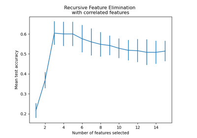
Recursive feature elimination with cross-validation